Descriptive Guide to CAP
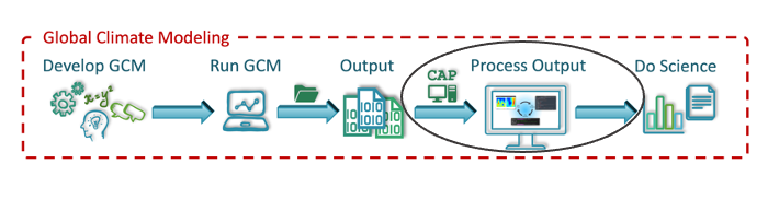
Table of Contents
CAP is a toolkit designed to simplify the post-processing of Mars Global Climate Model (MGCM) output. Written in Python, CAP works with existing Python libraries, allowing users to install and use it easily and free of charge. Without CAP, plotting MGCM output requires users to provide their own scripts for post-processing tasks such as interpolating the vertical grid, computing derived variables, converting between file types, and creating diagnostic plots.

Such a process requires users to be familiar with Fortran files and able to write scripts to perform file manipulations and create plots. CAP standardizes the post-processing effort by providing executables that can perform file manipulations and create diagnostic plots from the command line, enabling users of almost any skill level to post-process and plot MGCM data.

Key CAP Features
Python-based: Built with an open-source programming language with extensive scientific libraries
Virtual Environment: Provides cross-platform support (MacOS, Linux, Windows), robust version control, and non-intrusive installation
Modular Design: Composed of both libraries (functions) and five executables for efficient command-line processing
netCDF4 Format: Uses a self-descriptive data format widely employed in the climate modeling community
FV3 Format Convention: Follows formatting conventions from the GFDL Finite-Volume Cubed-Sphere Dynamical Core
Multi-model Support: Currently supports both NASA Ames Legacy GCM and NASA Ames GCM with the FV3 dynamical core, with planned expansion to other Global Climate Models
CAP Components
CAP consists of five executables:
MarsPull - Access MGCM output
MarsFiles - Reduce the files
MarsVars - Perform variable operations
MarsInterp - Interpolate the vertical grid
MarsPlot - Visualize the MGCM output
Cheat Sheet
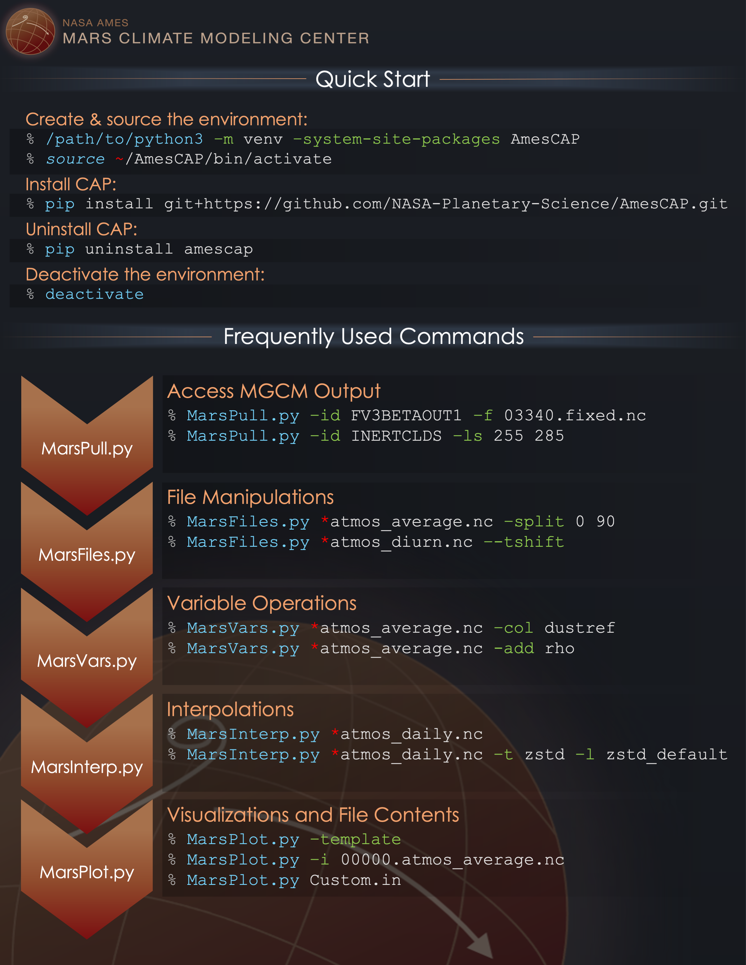
CAP is designed to be modular. Users can post-process and plot MGCM output exclusively with CAP or selectively integrate CAP into their own analysis routines.
Getting Help
Use the [-h --help] option with any executable to display documentation and examples:
(amesCAP)$ MarsPlot -h
> usage: MarsPlot [-h] [-i INSPECT_FILE] [-d DATE [DATE ...]] [--template]
>                   [-do DO] [-sy] [-o {pdf,eps,png}] [-vert] [-dir DIRECTORY]
>                   [--debug]
>                   [custom_file]
1. MarsPull - Downloading Raw MGCM Output
MarsPull is a utility for accessing MGCM output files hosted on the MCMC Data portal. MGCM data is archived in 1.5-hour intervals (16x/day) and packaged in files containing 10 sols. The files are named fort.11_XXXX in the order they were produced, but MarsPull maps those files to specific solar longitudes (Ls, in °).
This allows users to request a file at a specific Ls or for a range of Ls using the [-ls --ls] flag. MarsPull requires the name of the folder to parse files from, and folders can be listed using [-list --list_files]. The [-f --filename] flag can be used to parse specific files within a particular directory.
MarsPull INERTCLDS -ls 255 285
MarsPull ACTIVECLDS -f fort.11_0720 fort.11_0723
Return to Table of Contents
2. MarsFiles - File Manipulations and Reduction
MarsFiles provides several tools for file manipulations, reduction, filtering, and data extraction from MGCM outputs.
Files generated by the NASA Ames MGCM are in netCDF4 data format with different (runscript-customizable) binning options:
File name |
Description |
Timesteps for 10 sols x 24 output/sol |
Ratio to daily |
|---|---|---|---|
atmos_daily.nc |
Continuous time series |
(24 x 10)=240 |
1 |
atmos_diurn.nc |
Data binned by time of day and 5-day average |
(24 x 2)=48 |
x5 smaller |
atmos_average.nc | 5-day averages |
(1 x 2) = 2 |
x80 smaller |
|
fixed.nc |
Static variables (surface albedo, topography) |
static |
few kB |
Data Reduction Functions
Create multi-day averages of continuous time-series:
[-ba --bin_average]Create diurnal composites of continuous time-series:
[-bd --bin_diurn]Extract specific seasons from files:
[-split --split]Combine multiple files into one:
[-c --concatenate]Create zonally-averaged files:
[-za --zonal_average]

Data Transformation Functions
Perform tidal analysis on diurnal composite files:
[-tide --tide_decomp]Perform propagating tideal analysis on diurnal composite files:
[-prop --prop_tides]Apply temporal filters to time-varying fields:
Low pass:
[-lpt --low_pass_temporal]High-pass:
[-hpt --high_pass_temporal]Band-pass:
[-bpt --band_pass_temporal]
Regrid a file to a different spatio/temporal grid:
[-regrid --regrid_xy_to_match]Time-shift diurnal composite files to uniform local time:
[-t --time_shift]
For all operations, you can process selected variables within the file using [-incl --include].
Time Shifting Example
Time shifting allows you to interpolate diurnal composite files to the same local times at all longitudes, which is useful for comparing with orbital datasets that often provide data at specific local times (e.g., 3am and 3pm).
(AmesCAP)$ MarsFiles *.atmos_diurn.nc -t
(AmesCAP)$ MarsFiles *.atmos_diurn.nc -t '3. 15.'
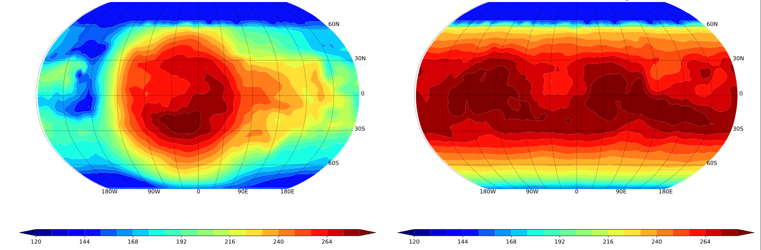
3pm surface temperature before (left) and after (right) processing a diurn file with MarsFiles to uniform local time (diurn_T.nc)
Return to Table of Contents
3. MarsVars - Performing Variable Operations
MarsVars provides tools for variable operations such as adding, removing, and modifying variables, and performing column integrations.
A typical use case is adding atmospheric density (rho) to a file. Because density is easily computed from pressure and temperature fields, it’s not archived in the GCM output to save space:
(amesCAP)$ MarsVars 00000.atmos_average.nc -add rho
You can verify the addition using MarsPlot’s [-i --inspect] function:
(amesCAP)$ MarsPlot -i 00000.atmos_average.nc
>
> ===================DIMENSIONS==========================
> ['bnds', 'time', 'lat', 'lon', 'pfull', 'scalar_axis', 'phalf']
> (etc)
> ====================CONTENT==========================
> pfull          : ('pfull',)= (30,), ref full pressure level  [Pa]
> temp           : ('time', 'pfull', 'lat', 'lon')= (4, 30, 180, 360), temperature  [K]
> rho            : ('time', 'pfull', 'lat', 'lon')= (4, 30, 180, 360), density (added postprocessing)  [kg/m3]
Available Variable Operations
Command Option |
Action |
|---|---|
-add –add_variable |
Add a variable to the file |
-rm –remove_variable |
Remove a variable from a file |
-extract –extract_copy |
Extract a list of variables to a new file |
-col –column_integrate |
Column integration, applicable to mixing ratios in [kg/kg] |
-zdiff –differentiate_wrt_z |
Vertical differentiation (e.g., compute gradients) |
-zd –zonal_detrend |
Zonally detrend a variable |
-edit –edit |
Change a variable’s name, attributes, or scale |
Example: Editing a NetCDF Variable
(AmesCAP)$ MarsVars *.atmos_average.nc -edit temp -rename airtemp
(AmesCAP)$ MarsVars *.atmos_average.nc -edit ps -multiply 0.01 -longname 'new pressure' -unit 'mbar'
Return to Table of Contents
4. MarsInterp - Interpolating the Vertical Grid
Native MGCM output files use a terrain-following pressure coordinate (pfull) as the vertical coordinate, meaning the geometric heights and actual mid-layer pressure of atmospheric layers vary based on location. For rigorous spatial averaging, it’s necessary to interpolate each vertical column to a standard pressure grid (_pstd grid):

Pressure interpolation from the reference pressure grid to a standard pressure grid
MarsInterp performs vertical interpolation from reference (pfull) layers to standard (pstd) layers:
(amesCAP)$ MarsInterp 00000.atmos_average.nc -t pstd
An inspection of the file shows that the pressure level axis has been replaced:
(amesCAP)$ MarsPlot -i 00000.atmos_average_pstd.nc
>
> ===================DIMENSIONS==========================
> ['bnds', 'time', 'lat', 'lon', 'scalar_axis', 'phalf', 'pstd']
> ====================CONTENT==========================
> pstd           : ('pstd',)= (36,), pressure  [Pa]
> temp           : ('time', 'pstd', 'lat', 'lon')= (4, 36, 180, 360), temperature  [K]
Interpolation Types
MarsInterp supports 3 types of vertical interpolation, selected with the [-t --interp_type] flag:
Command Option |
Description |
Lowest level value |
|---|---|---|
-t pstd |
Standard pressure [Pa] (default) |
1000 Pa |
-t zstd |
Standard altitude [m] |
-7000 m |
-t zagl |
Standard altitude above ground level [m] |
0 m |
Using Custom Vertical Grids
MarsInterp uses default grids for each interpolation type, but you can specify custom layers by editing the hidden file .amesgcm_profile in your home directory.
For first-time use, copy the template:
(amesCAP)$ cp ~/amesCAP/mars_templates/amesgcm_profile ~/.amesgcm_profile # Note the dot '.' !!!
Open ~/.amesgcm_profile with any text editor to see customizable grid definitions:
<<<<<<<<<<<<<<| Pressure definitions for pstd |>>>>>>>>>>>>>

p44=[1.0e+03, 9.5e+02, 9.0e+02, 8.5e+02, 8.0e+02, 7.5e+02, 7.0e+02,
     6.5e+02, 6.0e+02, 5.5e+02, 5.0e+02, 4.5e+02, 4.0e+02, 3.5e+02,
     3.0e+02, 2.5e+02, 2.0e+02, 1.5e+02, 1.0e+02, 7.0e+01, 5.0e+01,
     3.0e+01, 2.0e+01, 1.0e+01, 7.0e+00, 5.0e+00, 3.0e+00, 2.0e+00,
     1.0e+00, 5.0e-01, 3.0e-01, 2.0e-01, 1.0e-01, 5.0e-02, 3.0e-02,
     1.0e-02, 5.0e-03, 3.0e-03, 5.0e-04, 3.0e-04, 1.0e-04, 5.0e-05,
     3.0e-05, 1.0e-05]
Use your custom grid with the [-v --vertical_grid] argument:
(amesCAP)$ MarsInterp 00000.atmos_average.nc -t pstd -v phalf_mb
Return to Table of Contents
5. MarsPlot - Plotting the Results
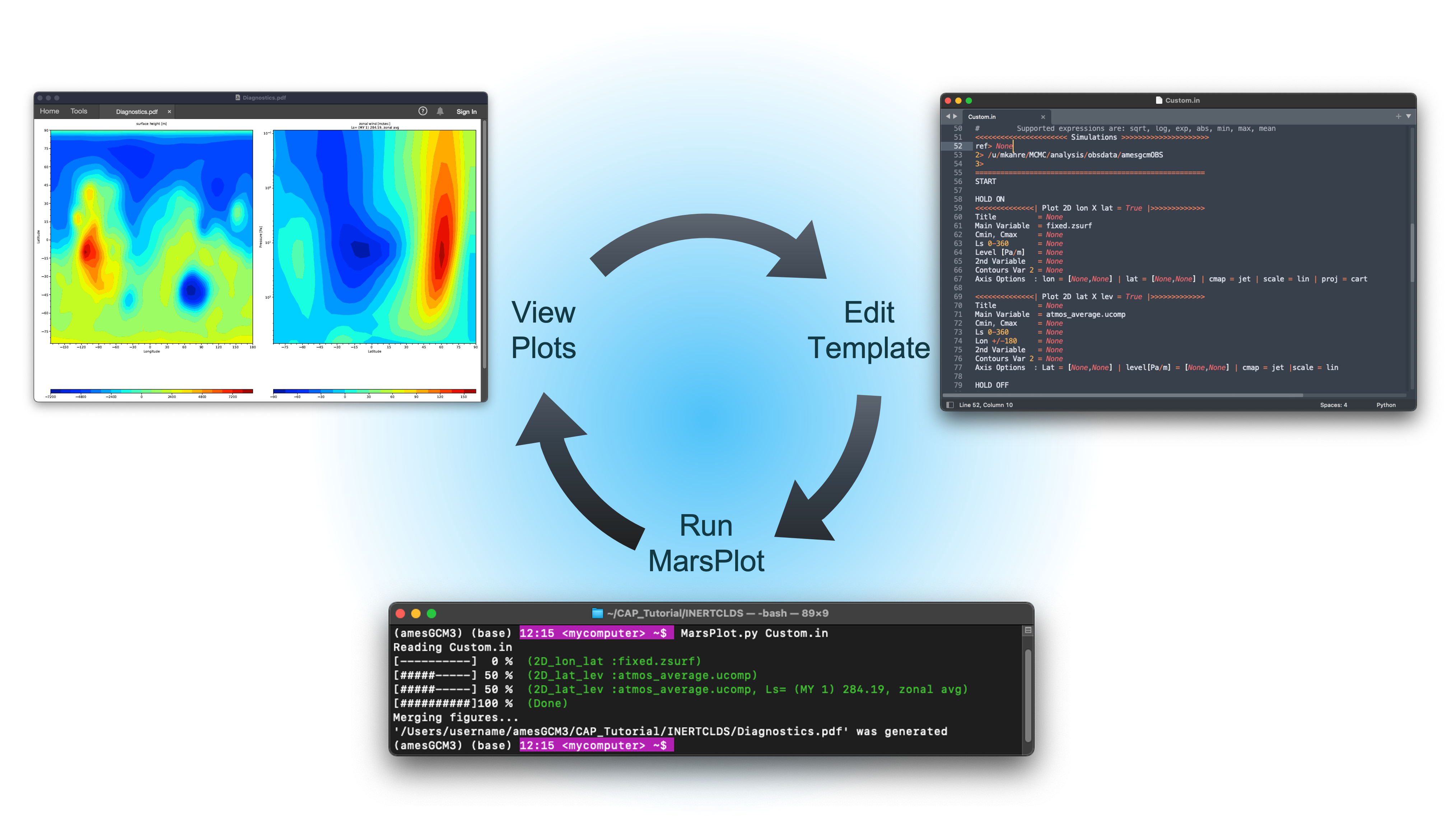
MarsPlot is CAP’s plotting routine. It accepts a modifiable template (Custom.in) containing a list of plots to create. Designed specifically for netCDF output files, it enables quick visualization of MGCM output.
The MarsPlot workflow involves three components:
MarsPlot in a terminal to inspect files and process the template
Custom.in template in a text editor
Diagnostics.pdf viewed in a PDF viewer
You can use MarsPlot to inspect netCDF files:
(amesCAP)> MarsPlot -i 07180.atmos_average.nc

> ===================DIMENSIONS==========================
> ['lat', 'lon', 'pfull', 'phalf', 'zgrid', 'scalar_axis', 'time']
> [...]
> ====================CONTENT==========================
> pfull          : ('pfull',)= (24,), ref full pressure level  [Pa]
> temp           : ('time', 'pfull', 'lat', 'lon')= (10, 24, 36, 60), temperature  [K]
> ucomp          : ('time', 'pfull', 'lat', 'lon')= (10, 24, 36, 60), zonal wind  [m/sec]
> [...]
Creating and Using a Template
Generate a template with the [-template --generate_template] argument:
(amesCAP)$ MarsPlot -template
> /path/to/simulation/run_name/history/Custom.in was created
(amesCAP)$
(amesCAP)$ MarsPlot Custom.in
> Reading Custom.in
> [----------]  0 % (2D_lon_lat :fixed.zsurf)
> [#####-----] 50 % (2D_lat_lev :atmos_average.ucomp, L\ :sub:`s`= (MY 2) 252.30, zonal avg)
> [##########]100 % (Done)
> Merging figures...
> /path/to/simulation/run_name/history/Diagnostics.pdf was generated
Plot Types and Cross-Sections
MarsPlot is designed to generate 2D cross-sections and 1D plots from multi-dimensional datasets. For this, you need to specify which dimensions to plot and which “free” dimensions to average/select.

A refresher on cross-sections for multi-dimensional datasets
The data selection process follows this decision tree:
1. Which simulation                                                 ┌─
   (e.g. ACTIVECLDS directory)                                      │  DEFAULT   1. ref> is current directory
         │                                                          │  SETTINGS
         └── 2. Which XXXXX start date                              │            2. latest XXXXX.fixed in directory
              (e.g. 00668, 07180)                                   └─
                  │                                                 ┌─
                  └── 3. Which type of file                         │
                       (e.g. diurn, average_pstd)                   │   USER     3. provided by user
                           │                                        │ PROVIDES
                           └── 4. Which variable                    │            4. provided by user
                                 (e.g. temp, ucomp)                 └─
                                   │                                ┌─
                                   └── 5. Which dimensions          │            5. see rule table below
                                      (e.g lat =0°,L\ :sub:`s` =270°)        │  DEFAULT
                                          │                         │  SETTINGS
                                          └── 6. plot customization │            6. default settings
                                                 (e.g. colormap)    └─
Default Settings for Free Dimensions
Free Dimension |
Default Setting |
Implementation |
|---|---|---|
time |
Last (most recent) timestep |
time = last timestep |
level |
Surface |
level = sfc |
latitude |
Equator |
lat = 0 (equator) |
longitude |
Zonal average |
lon = all (average ‘all’ longitudes) |
time of day |
3 pm (diurn files only) |
tod = 15 |
Custom.in Template Example
Here’s an example of a code snippet in Custom.in for a lon/lat cross-section:
<<<<<<<<<<<<<<| Plot 2D lon X lat = True |>>>>>>>>>>>>>
Title          = None
Main Variable  = atmos_average.temp
Cmin, Cmax     = None
Ls 0-360       = None
Level [Pa/m]   = None
2nd Variable   = None
Contours Var 2 = None
Axis Options  : lon = [None,None] | lat = [None,None] | cmap = jet | scale = lin | proj = cart
This plots the air temperature (temp) from the atmos_average.nc file as a lon/lat map. Since time and altitude are unspecified (set to None), MarsPlot will show the last timestep in the file and the layer adjacent to the surface.
Specifying Free Dimensions
Here are the accepted values for free dimensions:
Accepted Input |
Meaning |
Example |
|---|---|---|
|
Default settings |
|
|
Return index closest to requested |
|
|
|
|
|
Average over all dimension values |
|
* Whether the value is interpreted in Pa or m depends on the vertical coordinate of the file
Note
Time of day (tod) in diurn files is specified using brackets {} in the variable name, e.g.: Main Variable = atmos_diurn.temp{tod=15,18} for the average between 3pm and 6pm.
Return to Table of Contents
6. MarsPlot - File Analysis
Inspecting Variable Content of netCDF Files
The [-i --inspect] function can be combined with the [-values --print_values] flag to print variable values:
(amesCAP)$ MarsPlot -i 07180.atmos_average.nc -values pfull
> pfull=
> [8.7662227e-02 2.5499690e-01 5.4266089e-01 1.0518962e+00 1.9545468e+00
> 3.5580616e+00 6.2466631e+00 1.0509957e+01 1.7400265e+01 2.8756382e+01
> 4.7480076e+01 7.8348366e+01 1.2924281e+02 2.0770235e+02 3.0938846e+02
> 4.1609518e+02 5.1308148e+02 5.9254102e+02 6.4705731e+02 6.7754218e+02
> 6.9152936e+02 6.9731799e+02 6.9994830e+02 7.0082477e+02]
For large arrays, the [-stats --statistics] flag is more suitable. You can also request specific array indexes:
(amesCAP)$ MarsPlot -i 07180.atmos_average.nc -stats ucomp temp[:,-1,:,:]
_________________________________________________________________
  VAR            |      MIN      |      MEAN     |      MAX      |
_________________|_______________|_______________|_______________|
            ucomp|        -102.98|        6.99949|        192.088|
   temp[:,-1,:,:]|        149.016|        202.508|         251.05|
_________________|_______________|_______________|_______________|
Note
-1 refers to the last element in that axis, following Python’s indexing convention.
Disabling or Adding a New Plot
Code blocks set to = True instruct MarsPlot to draw those plots. Templates set to = False are skipped. MarsPlot supports seven plot types:
<<<<<| Plot 2D lon X lat  = True |>>>>>
<<<<<| Plot 2D lon X time = True |>>>>>
<<<<<| Plot 2D lon X lev  = True |>>>>>
<<<<<| Plot 2D lat X lev  = True |>>>>>
<<<<<| Plot 2D time X lat = True |>>>>>
<<<<<| Plot 2D time X lev = True |>>>>>
<<<<<| Plot 1D            = True |>>>>> # Any 1D Plot Type (Dimension x Variable)
Adjusting the Color Range and Colormap
Cmin, Cmax sets the contour range for shaded contours, while Contours Var 2 does the same for solid contours. Two values create a range with 24 evenly-spaced contours; more values define specific contour levels:
Main Variable  = atmos_average.temp     # filename.variable *REQUIRED
Cmin, Cmax     = 240,290                # Colorbar limits (minimum, maximum)
2nd Variable   = atmos_average.ucomp    # Overplot U winds
Contours Var 2 = -200,-100,100,200      # List of contours for 2nd Variable or CMIN, CMAX
Axis Options  : Ls = [None,None] | lat = [None,None] | cmap = jet |scale = lin
Contour spacing can be linear (scale = lin) or logarithmic (scale = log) for values spanning multiple orders of magnitude.
You can change the colormap from the default cmap = jet to any Matplotlib colormap:

Add the _r suffix to reverse a colormap (e.g., cmap = jet_r for red-to-blue instead of blue-to-red).
Creating 1D Plots
The 1D plot template differs from other templates:
Uses
Legendinstead ofTitleto label plots when overplotting multiple variablesIncludes additional
linestyleaxis optionsHas a
Diurnaloption that can only beNoneorAXIS
<<<<<<<<<<<<<<| Plot 1D = True |>>>>>>>>>>>>>
Legend         = None                   # Legend instead of Title
Main Variable  = atmos_average.temp
Ls 0-360       = AXIS                   # Any of these can be selected
Latitude       = None                   # as the X axis dimension, and
Lon +/-180     = None                   # the free dimensions can accept
Level [Pa/m]   = None                   # values as before. However,
Diurnal  [hr]  = None                   # ** Diurnal can ONLY be AXIS or None **
Customizing 1D Plots
Axis Options controls axes limits and linestyle for 1D plots:
1D Plot Option |
Usage |
Example |
|---|---|---|
|
X or Y axes range depending on plot type |
|
|
Plotted variable range |
|
|
Linestyle (Matplotlib convention) |
|
|
Name for the variable axis |
|
Available colors, linestyles, and marker styles for 1D plots:

Putting Multiple Plots on the Same Page
Use HOLD ON and HOLD OFF to group figures on the same page:
HOLD ON

<<<<<<| Plot 2D lon X lat = True |>>>>>>
Title    = Surface CO2 Ice (g/m2)
.. (etc) ..

<<<<<<| Plot 2D lon X lat = True |>>>>>>
Title    = Surface Wind Speed (m/s)
.. (etc) ..

HOLD OFF
By default, MarsPlot will arrange the plots automatically. Specify a custom layout with HOLD ON rows,columns (e.g., HOLD ON 4,3).
Putting Multiple 1D Plots on the Same Page
Use ADD LINE between templates to place multiple 1D plots on the same figure:
<<<<<<| Plot 1D = True |>>>>>>
Main Variable    = var1
.. (etc) ..

ADD LINE

<<<<<<| Plot 1D = True |>>>>>>
Main Variable    = var2
.. (etc) ..
Note
When combining HOLD ON/HOLD OFF with ADD LINE on a multi-figure page, the 1D plot with sub-plots must be the LAST one on that page.
Using a Different Start Date
For simulations with multiple files of the same type:
00000.fixed.nc          00100.fixed.nc         00200.fixed.nc         00300.fixed.nc
00000.atmos_average.nc  00100.atmos_average.nc 00200.atmos_average.nc 00300.atmos_average.nc
By default, MarsPlot uses the most recent files (e.g., 00300.fixed.nc and 00300.atmos_average.nc). Instead of specifying dates in each Main Variable entry, use the -date argument:
MarsPlot Custom.in -d 200
You can also specify a range of sols: MarsPlot Custom.in -d 100 300
For 1D plots spanning multiple years, use [-sy --stack_years] to overplot consecutive years instead of showing them sequentially.
Accessing Simulations in Different Directories
The <<< Simulations >>> block at the beginning of Custom.in lets you point to different directories:
<<<<<<<<<<<<<<<<<<<<<< Simulations >>>>>>>>>>>>>>>>>>>>>
ref> None
2> /path/to/another/sim # another simulation
3>
=======================================================
When ref> is set to None, it refers to the current directory. Access variables from other directories using the @ symbol:
Main Variable = XXXXX.filename@N.variable
Where N is the simulation number from the <<< Simulations >>> block.
Overwriting Free Dimensions
By default, MarsPlot applies the free dimensions specified in the template to both Main Variable and 2nd Variable. Override this using curly braces {} with a semicolon-separated list of dimensions:
<<<<<<<<<<<<<<| Plot 2D lon X lat = True |>>>>>>>>>>>>>
...
Main Variable  = atmos_average.var
...
Ls 0-360       = 270
Level [Pa/m]   = 10
2nd Variable   = atmos_average.var{ls=90,180;lev=50}
Here, Main Variable uses Ls`=270° and pressure=10 Pa, while ``2nd Variable` uses the average of L:sub:`s`=90-180° and pressure=50 Pa.
Note
Dimension keywords are ls, lev, lon, lat, and tod. Accepted values are Value (closest), Valmin,Valmax (average between two values), and all (average over all values).
Performing Element-wise Operations
Use square brackets [] for element-wise operations:
# Convert topography from meters to kilometers
Main Variable = [fixed.zsurf]/(10.**3)

# Normalize dust opacity
Main Variable = [atmos_average.taudust_IR]/[atmos_average.ps]*610

# Temperature difference between reference simulation and simulation 2
Main Variable = [atmos_average.temp]-[atmos_average@2.temp]

# Temperature difference between surface and 10 Pa level
Main Variable = [atmos_average.temp]-[atmos_average.temp{lev=10}]
Using Code Comments and Speeding Up Processing
Use # for comments (following Python convention). Each block must remain intact, so add comments between templates or comment all lines of a template.
The START keyword at the beginning of Custom.in tells MarsPlot where to begin parsing templates:
=======================================================
START
To skip processing certain plots, move the START keyword further down instead of individually setting plots to False. You can also add a STOP keyword to process only plots between START and STOP.
Changing Projections
For Plot 2D lon X lat figures, MarsPlot supports multiple projections:
Cylindrical projections:
cart(cartesian)robin(robinson)moll(mollweide)
Azimuthal projections:
Npole(north polar)Spole(south polar)ortho(orthographic)

(Top) cylindrical projections: cart, robin, and moll. (Bottom) azimuthal projections: Npole, Spole, and ortho
Azimuthal projections accept optional arguments:
# Zoom in/out on the North pole
proj = Npole lat_max

# Zoom in/out on the South pole
proj = Spole lat_min

# Rotate the globe
proj = ortho lon_center, lat_center
Adjusting Figure Format and Size
Change the output format with
[-ftype --figure_filetype]: choose between pdf (default), png, or epsAdjust page width with
[-pw --pixel_width](default: 2000 pixels)Switch to portrait orientation with
[-portrait --portrait_mode]
Accessing CAP Libraries for Custom Plots
CAP libraries are available for custom analysis:
Core utilities:
amescap/FV3_utilsSpectral utilities:
amescap/Spectral_utilsFile parsing classes:
amescap/Ncdf_wrapper
Example of using CAP libraries for custom analysis:
# Import python packages
import numpy as np # for array operations
import matplotlib.pyplot as plt # python plotting library
from netCDF4 import Dataset # to read .nc files

# Open a dataset and read the 'variables' attribute from the NETCDF FILE
nc_file = Dataset('/path/to/00000.atmos_average_pstd.nc', 'r')

vars_list = nc_file.variables.keys()
print('The variables in the atmos files are: ', vars_list)

lon = nc_file.variables['lon'][:]
lat = nc_file.variables['lat'][:]

# Read the 'shape' and 'units' attribute from the temperature VARIABLE
file_dims = nc_file.variables['temp'].shape
units_txt = nc_file.variables['temp'].units
print(f'The data dimensions are {file_dims}')

# Read the pressure, time, and the temperature for an equatorial cross section
pstd = nc_file.variables['pstd'][:]
areo = nc_file.variables['areo'][0] # solar longitude for the 1st timestep
temp = nc_file.variables['temp'][0,:,18,:] # time, press, lat, lon
nc_file.close()

# Get the latitude of the cross section.
lat_cross = lat[18]

# Example of accessing functions from the Ames Pipeline if we wanted to plot
# the data in a different coordinate system (0>360 instead of +/-180 )

from amescap.FV3_utils import lon180_to_360, shiftgrid_180_to_360

lon360 = lon180_to_360(lon)
temp360 = shiftgrid_180_to_360(lon, temp)

# Define some contours for plotting
contours = np.linspace(150, 250, 32)

# Create a figure with the data
plt.close('all')
ax = plt.subplot(111)
plt.contourf(lon, pstd, temp, contours, cmap='jet', extend='both')
plt.colorbar()

# Axis labeling
ax.invert_yaxis()
ax.set_yscale("log")
plt.xlabel('Longitudes')
plt.ylabel('Pressure [Pa]')
plt.title(f'Temperature [{units_txt}] at Ls = {areo}, lat = {lat_cross}')
plt.show()
Debugging
MarsPlot handles missing data and many errors internally, reporting issues in the terminal and in the generated figures. To get standard Python errors during debugging, use the --debug option, which will raise errors and stop execution.
Note
Errors raised with the --debug flag may reference MarsPlot’s internal classes, so they may not always be self-explanatory.
Return to Table of Contents