Examples & Use Cases

CAP is a Python toolkit designed to simplify post-processing and plotting MGCM output. CAP consists of five Python executables:

1. MarsPull → accessing MGCM output

2. MarsFiles → reducing the files

3. MarsVars → performing variable operations

4. MarsInterp → interpolating the vertical grid

5. MarsPlot → plotting MGCM output

The following exercises are organized into two parts by function.

Part I: File Manipulations → MarsFiles, MarsVars, & MarsInterp

Part II: Plotting with CAP → MarsPlot

Note

This does not cover MarsPull.

---

Table of Contents

• Activating CAP

• Part I: File Manipulations - 1. MarsPlot’s Inspect Function - 2. Editing Variable Names and Attributes - 3. Splitting Files in Time - 4. Deriving Secondary Variables - 5. Time-Shifting Diurn Files - 6. Pressure-Interpolating the Vertical Axis

• Part II: Plotting with CAP - Step 1: Creating the Template (Custom.in) - Step 2: Editing Custom.in - Step 3: Generating the Plots

• Custom Set 1 of 4: Zonal Mean Surface Plots Over Time

• Custom Set 2 of 4: Global Mean Column-Integrated Dust Optical Depth Over Time

• Custom Set 3 of 4: 50 Pa Temperatures at 3 AM and 3 PM

• Custom Set 4 of 4: Zonal Mean Circulation Cross-Sections

---

Activating CAP

Activate the amescap virtual environment to use CAP:

(local)~$ source ~/amescap/bin/activate
(amescap)~$

Confirm that CAP’s executables are accessible by typing [-h --help], which prints documentation for the executable to the terminal:

(amescap)~$ MarsVars -h

Now that we know CAP is configured, make a copy of the file amescap_profile in your home directory, and make it a hidden file:

(amescap)~$ cp ~/amescap/mars_templates/amescap_profile ~/.amescap_profile

CAP stores useful settings in amescap_profile. Copying it to our home directory ensures it is not overwritten if CAP is updated or reinstalled.

Part I covers file manipulations. Some exercises build off of previous exercises so it is important to complete them in order. If you make a mistake or get behind in the process, you can go back and catch up during a break or use the provided answer key before continuing on to Part II.

Part II demonstrates CAP’s plotting routine. There is more flexibility in this part of the exercise.

Return to Table of Contents

Part I: File Manipulations

CAP has dozens of post-processing capabilities. We will go over a few of the most commonly used functions in this tutorial. We will cover:

• Interpolating data to different vertical coordinate systems (MarsInterp)

• Adding derived variables to the files (MarsVars)

• Time-shifting data to target local times (MarsFiles)

• Trimming a file to reduce its size (MarsFiles).

The required MGCM output files are already loaded in the cloud environment under tutorial_files/cap_exercises/. Change to that directory and look at the contents:

(amescap)~$ cd tutorial_files/cap_exercises
(amescap)~$ ls
03340.atmos_average.nc  03340.backup.zip
03340.atmos_diurn.nc    03340.fixed.nc

The three MGCM output files have a 5-digit sol number appended to the front of the file name. The sol number indicates the day that a file’s record begins. These contain output from the sixth year of a simulation. The zipped file is an archive of these three output files in case you need it.

Note

The output files we manipulate in Part I will be used to generating plots in Part II so do not delete any file you create!

1. MarsPlot’s Inspect Function

The inspect function is part of MarsPlot and it prints netCDF file contents to the screen. To use it on the average file, 03340.atmos_average.nc, type the following in the terminal:

(amescap)~$ MarsPlot -i 03340.atmos_average.nc

Note

This is a good time to remind you that if you are unsure how to use a function, invoke the [-h --help] argument with any executable to see its documentation (e.g., MarsPlot -h).

Return to Part I: File Manipulations

---

2. Editing Variable Names and Attributes

In the previous exercise, [-i --inspect] revealed a variable called opac in 03340.atmos_average.nc. opac is dust opacity per pascal and it is similar to another variable in the file, dustref, which is opacity per (model) level. Let’s rename opac to dustref_per_pa to better indicate the relationship between these variables.

We can modify variable names, units, longnames, and even scale variables using the [-edit --edit] function in MarsVars. The syntax for editing the variable name is:

(amescap)~$ MarsVars 03340.atmos_average.nc -edit opac -rename dustref_per_pa
03340.atmos_average_tmp.nc was created
03340.atmos_average.nc was updated

We can use [-i --inspect] again to confirm that opac was renamed dustref_per_pa:

(amescap)~$ MarsPlot -i 03340.atmos_average.nc

The [-i --inspect] function can also print a summary of the values of a variable to the screen using [-stats --statistics]. For example:

(amescap)~$ MarsPlot -i 03340.atmos_average.nc -stats dustref_per_pa
_________________________________________________________
  VAR           |   MIN     |    MEAN     |    MAX      |
________________|___________|_____________|_____________|
  dustref_per_pa|          0|  0.000384902|    0.0017573|
________________|___________|_____________|_____________|

Finally, [-i --inspect] can print the values of a variable to the screen using [-values --print_values]. For example:

(amescap)~$ MarsPlot -i 03340.atmos_average.nc -values lat
lat=
[-89. -87. -85. -83. -81. -79. -77. -75. -73. -71. -69. -67. -65. -63.
 -61. -59. -57. -55. -53. -51. -49. -47. -45. -43. -41. -39. -37. -35.
 -33. -31. -29. -27. -25. -23. -21. -19. -17. -15. -13. -11.  -9.  -7.
  -5.  -3.  -1.   1.   3.   5.   7.   9.  11.  13.  15.  17.  19.  21.
  1.   25.  27.  29.  31.  33.  35.  37.  39.  41.  43.  45.  47.  49.
  2.   53.  55.  57.  59.  61.  63.  65.  67.  69.  71.  73.  75.  77.
  3.   81.  83.  85.  87.  89.]

Return to Part I: File Manipulations

---

3. Splitting Files in Time

Next we’re going to trim the diurn and average files by L_s. We’ll create files that only contain data around southern summer solstice, L_s=270. This greatly reduces the file size to make our next post-processing steps more efficient.

Syntax for trimming files by L_suses [-split --split]:

(amescap)~$ MarsFiles 03340.atmos_diurn.nc -split 265 275
...
/home/centos/tutorial_files/cap_exercises/03847.atmos_diurn_Ls265_275.nc was created

(amescap)~$ MarsFiles 03340.atmos_average.nc -split 265 275
...
/home/centos/tutorial_files/cap_exercises/03847.atmos_average_Ls265_275.nc was created

The trimmed files have the appendix _Ls265_275.nc and the simulation day has changed from 03340 to 03847 to reflect that the first day in the file has changed.

For future steps, we need a fixed file with the same simulation day number as the files we just created, so make a copy of the fixed file and rename it:

(amescap)~$ cp 03340.fixed.nc 03847.fixed.nc

Return to Part I: File Manipulations

---

4. Deriving Secondary Variables

The [-add --add_variable] function in MarsVars derives and adds secondary variables to MGCM output files provided that the variable(s) required for the derivation are already in the file. We will add the meridional mass streamfunction (msf) to the trimmed average file. To figure out what we need in order to do this, use the [-h --help] function on MarsVars:

(amescap)~$ MarsVars -h

The help function shows that streamfunction (msf) requires two things: that the meridional wind (vcomp) is in the average file, and that the average file is *pressure-interpolated*.

First, confirm that vcomp is in 03847.atmos_average_Ls265_275.nc using [-i --inspect]:

(amescap)~$ MarsPlot -i 03847.atmos_average_Ls265_275.nc
...
vcomp : ('time', 'pfull', 'lat', 'lon')= (3, 56, 90, 180), meridional wind  [m/sec]

Second, pressure-interpolate the average file using MarsInterp. The call to MarsInterp requires:

• The interpolation type ([-t --interp_type]), we will use standard pressure coorindates (pstd)

• The grid to interpolate to ([--v --vertical_grid]), we will use the default pressure grid (pstd_default)

Note

All interpolation types are listed in the [-h --help] documentation for MarsInterp. Additional grids are listed in ~/.amescap_profile, which accepts user-input grids as well.

We will also specify that only temperature (temp), winds (ucomp and vcomp), and surface pressure (ps) are to be included in this new file using [-incl --include]. This will reduce the interpolated file size.

Finally, add the [-print --print_grid] flag at the end of prompt to print out the standard pressure grid levels that we are interpolating to:

(amescap)~$ MarsInterp 03847.atmos_average_Ls265_275.nc -t pstd -v pstd_default -incl temp ucomp vcomp ps -print
1100.0 1050.0 1000.0 950.0 900.0 850.0 800.0 750.0 700.0 650.0 600.0 550.0 500.0 450.0 400.0 350.0 300.0 250.0 200.0 150.0 100.0 70.0 50.0 30.0 20.0 10.0 7.0 5.0 3.0 2.0 1.0 0.5 0.3 0.2 0.1 0.05

To perform the interpolation, simply omit the [-print --print_grid] flag:

(amescap)~$ MarsInterp 03847.atmos_average_Ls265_275.nc -t pstd -v pstd_default -incl temp ucomp vcomp ps
...
/home/centos/tutorial_files/cap_exercises/03847.atmos_average_Ls265_275_pstd.nc was created

Now we have a pressure-interpolated average file with vcomp in it. We can derive and add msf to it using [-add --add_variable] from MarsVars:

(amescap)~$ MarsVars 03847.atmos_average_Ls265_275_pstd.nc -add msf
Processing: msf...
msf: Done

Return to Part I: File Manipulations

---

5. Time-Shifting Diurn Files

The diurn file is organized by time-of-day assuming *universal* time starting at the Martian prime meridian. The time-shift [-t --time_shift] function interpolates the diurn file to *uniform local* time. This is especially useful when comparing MGCM output to satellite observations in fixed local time orbit.

Time-shifting can only be done on files with a local time dimension (time_of_day_24, i.e. diurn files). By default, MarsFiles time shifts all of the data in the file to 24 uniform local times and this generates very large files. To reduce file size and processing time, we will time-shift the data only to the local times we are interested in: 3 AM and 3 PM.

Time-shift the temperature (temp) and surface pressure (ps) in the trimmed diurn file to 3 AM / 3 PM local time like so:

(amescap)~$ MarsFiles 03847.atmos_diurn_Ls265_275.nc -t '3. 15.' -incl temp ps
...
/home/centos/tutorial_files/cap_exercises/03847.atmos_diurn_Ls265_275_T.nc was created

A new diurn file called 03847.atmos_diurn_Ls265_275_T.nc is created. Use [-i --inspect] to confirm that only ps and temp (and their dimensions) are in the file and that the time_of_day dimension has a length of 2:

(amescap)~$ MarsPlot -i 03847.atmos_diurn_Ls265_275_T.nc
...
====================CONTENT==========================
time           : ('time',)= (3,), sol number  [days since 0000-00-00 00:00:00]
time_of_day_02 : ('time_of_day_02',)= (2,), time of day  [[hours since 0000-00-00 00:00:00]]
pfull          : ('pfull',)= (56,), ref full pressure level  [mb]
scalar_axis    : ('scalar_axis',)= (1,), none  [none]
lon            : ('lon',)= (180,), longitude  [degrees_E]
lat            : ('lat',)= (90,), latitude  [degrees_N]
areo           : ('time', 'time_of_day_02', 'scalar_axis')= (3, 2, 1), areo  [degrees]
ps             : ('time', 'time_of_day_02', 'lat', 'lon')= (3, 2, 90, 180), surface pressure  [Pa]
temp           : ('time', 'time_of_day_02', 'pfull', 'lat', 'lon')= (3, 2, 56, 90, 180), temperature  [K]
=====================================================

Return to Part I: File Manipulations

---

6. Pressure-Interpolating the Vertical Axis

Now we can efficiently interpolate the diurn file to the standard pressure grid. Recall that interpolation is part of MarsInterp and requires:

1. Interpolation type ([-t --interp_type]), and

2. Grid ([-v --vertical_grid])

As before, we will interpolate to standard pressure (pstd) using the default pressure grid in .amesgcm_profile (pstd_default):

(amescap)~$ MarsInterp 03847.atmos_diurn_Ls265_275_T.nc -t pstd -v pstd_default
...
/home/centos/tutorial_files/cap_exercises/03847.atmos_diurn_Ls265_275_T_pstd.nc was created

Note

Interpolation could be done before or after time-shifting, the order does not matter.

We now have four different diurn files in our directory:

03340.atmos_diurn.nc                  # Original MGCM file
03847.atmos_diurn_Ls265_275.nc        # + Trimmed to L$_s$=240-300
03847.atmos_diurn_Ls265_275_T.nc      # + Time-shifted; `ps` and `temp` only
03847.atmos_diurn_Ls265_275_T_pstd.nc # + Pressure-interpolated

CAP always adds an appendix to the name of any new file it creates. This helps users keep track of what was done and in what order. The last file we created was trimmed, time-shifted, then pressure-interpolated. However, the same file could be generated by performing the three functions in any order.

Return to Part I: File Manipulations

Part II

This part of the CAP Practical covers how to generate plots with CAP. We will take a learn-by-doing approach, creating five sets of plots that demonstrate some of CAP’s most often used plotting capabilities:

1. Custom Set 1 of 4: Zonal Mean Surface Plots Over Time

2. Custom Set 2 of 4: Global Mean Column-Integrated Dust Optical Depth Over Time

3. Custom Set 3 of 4: 50 Pa Temperatures at 3 AM and 3 PM

4. Custom Set 4 of 4: Zonal Mean Circulation Cross-Sections

Plotting with CAP is done in 3 steps:

Step 1: Creating the Template (Custom.in)

Step 2: Editing Custom.in

Step 3: Generating the Plots

As in Part I, we will go through these steps together.

Part II: Plotting with CAP

CAP’s plotting routine is MarsPlot. It works by generating a Custom.in file containing seven different plot templates that users can modify, then reading the Custom.in file to make the plots.

The plot templates in Custom.in include:

Plot Type	X, Y Dimensions	Name in Custom.in
Map	Longitude, Latitude	Plot 2D lon x lat
Time-varying	Time, Latitude	Plot 2D time x lat
Time-varying	Time, level	Plot 2D time x lev
Time-varying	Longitude, Time	Plot 2D lon x time
Cross-section	Longitude, Level	Plot 2D lon x lev
Cross-section	Latitude, Level	Plot 2D lat x lev
Line plot (1D)	Dimension*, Variable	Plot 1D

Note

Dimension is user-indicated and could be time (time), latitude (lat), longitude lon, or level (pfull, pstd, zstd, zagl).

Additionally, MarsPlot supports:

• PDF & image format

• Landscape & portrait mode

• Multi-panel plots

• Overplotting

• Customizable axes dimensions and contour intervals

• Adjustable colormaps and map projections

and so much more. You will learn to plot with MarsPlot by following along with the demonstration. We will generate the Custom.in template file, customize it, and pass it back into MarsPlot to create plots.

Return to Part II

---

Step 1: Creating the Template (Custom.in)

Generate the template file using [-template --generate_template], Custom.in:

(amescap)~$ MarsPlot -template
/home/centos/tutorial_files/cap_exercises/Custom.in was created

A new file called Custom.in is created in your current working directory.

---

Step 2: Editing Custom.in

Open Custom.in using vim:

(amescap)~$ vim Custom.in

Scroll down until you see the first two templates shown in the image below:

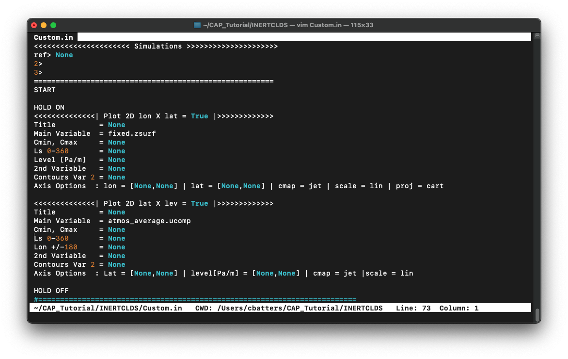
Since all of the templates have a similar structure, we can broadly describe how Custom.in works by going through the templates line-by-line.

Line 1

# Line 1                ┌ plot type  ┌ whether to create the plot
<<<<<<<<<<<<<<| Plot 2D lon X lat = True |>>>>>>>>>>>>>

Line 1 indicates the plot type and whether to create the plot when passed into MarsPlot.

Line 2

# Line 2         ┌ title
Title          = None

Line 2 is where we set the plot title.

Line 3

# Line 3         ┌ file ┌ variable
Main Variable  = fixed.zsurf          # file.variable
Main Variable  = [fixed.zsurf]/1000   # [] brackets for mathematical operations
Main Variable  = diurn_T.temp{tod=3}  # {} brackets for dimension selection

Line 3 indicates the variable to plot and the file from which to pull the variable.

Additional customizations include:

• Element-wise operations (e.g., scaling by a factor)

• Dimensional selection (e.g., selecting the time of day (tod) at which to plot from a time-shifted diurn file)

Line 4

# Line 4
Cmin, Cmax     = None           # automatic, or
Cmin, Cmax     = -4,5           # contour limits, or
Cmin, Cmax     = -4,-2,0,1,3,5  # explicit contour levels

Line 4 line defines the color-filled contours for Main Variable. Valid inputs are:

• None (default) enables Python’s automatic interpretation of the contours

• min,max specifies contour range

• X,Y,Z,...,N gives explicit contour levels

Lines 5 & 6

# Lines 5 & 6
Ls 0-360       = None # for 'time' free dimension
Level Pa/m     = None # for 'pstd' free dimension

Lines 5 & 6 handle the free dimension(s) for Main Variable (the dimensions that are *not* plot dimensions).

For example, temperature has four dimensions: (time, pstd, lat, lon). For a 2D lon X lat map of temperature, lon and lat provide the x and y dimensions of the plot. The free dimensions are then pstd (Level Pa/m) and time (Ls 0-360).

Lines 5 & 6 accept four input types:

1. integer selects the closest value

2. min,max averages over a range of the dimension

3. all averages over the entire dimension

4. None (default) depends on the free dimension:

# ┌ free dimension  ┌ default setting
Ls 0-360       = None   # most recent timestep
Level Pa/m     = None   # surface level
Lon +/-180     = None   # zonal mean over all longitudes
Latitude       = None   # equatorial values only

Lines 7 & 8

# Line 7 & 8
2nd Variable   = None           # no solid contours
2nd Variable   = fixed.zsurf    # draw solid contours
Contours Var 2  = -4,5          # contour range, or
Contours Var 2  = -4,-2,0,1,3,5 # explicit contour levels

Lines 7 & 8 (optional) define the solid contours on the plot. Contours can be drawn for Main Variable or a different 2nd Variable.

• Like Main Variable, 2nd Variable minimally requires file.variable

• Like Cmin, Cmax, Contours Var 2 accepts a range (min,max) or list of explicit contour levels (X,Y,Z,...,N)

Line 9

# Line 9        ┌ X axes limit      ┌ Y axes limit      ┌ colormap   ┌ cmap scale  ┌ projection
 Axis Options : lon = [None,None] | lat = [None,None] | cmap = jet | scale = lin | proj = cart

Finally, Line 9 offers plot customization (e.g., axes limits, colormaps, map projections, linestyles, 1D axes labels).

Return to Part II

---

Step 3: Generating the Plots

Generate the plots set to True in Custom.in by saving and quitting the editor (:wq) and then passing the template file to MarsPlot. The first time we do this, we’ll pass the [-d --date] flag to specify that we want to plot from the 03340 average and fixed files:

(amescap)~$ MarsPlot Custom.in -d 03340

Plots are created and saved in a file called Diagnostics.pdf.

---

Summary

Plotting with MarsPlot is done in 3 steps:

(amescap)~$ MarsPlot -template # generate Custom.in
(amescap)~$ vim Custom.in # edit Custom.in
(amescap)~$ MarsPlot Custom.in # pass Custom.in back to MarsPlot

Now we will go through some examples.

---

Customizing the Plots

Open Custom.in in the editor:

(amescap)~$ vim Custom.in

Copy the first two templates that are set to True and paste them below the line Empty Templates (set to False). Then, set them to False. This way, we have all available templates saved at the bottom of the script.

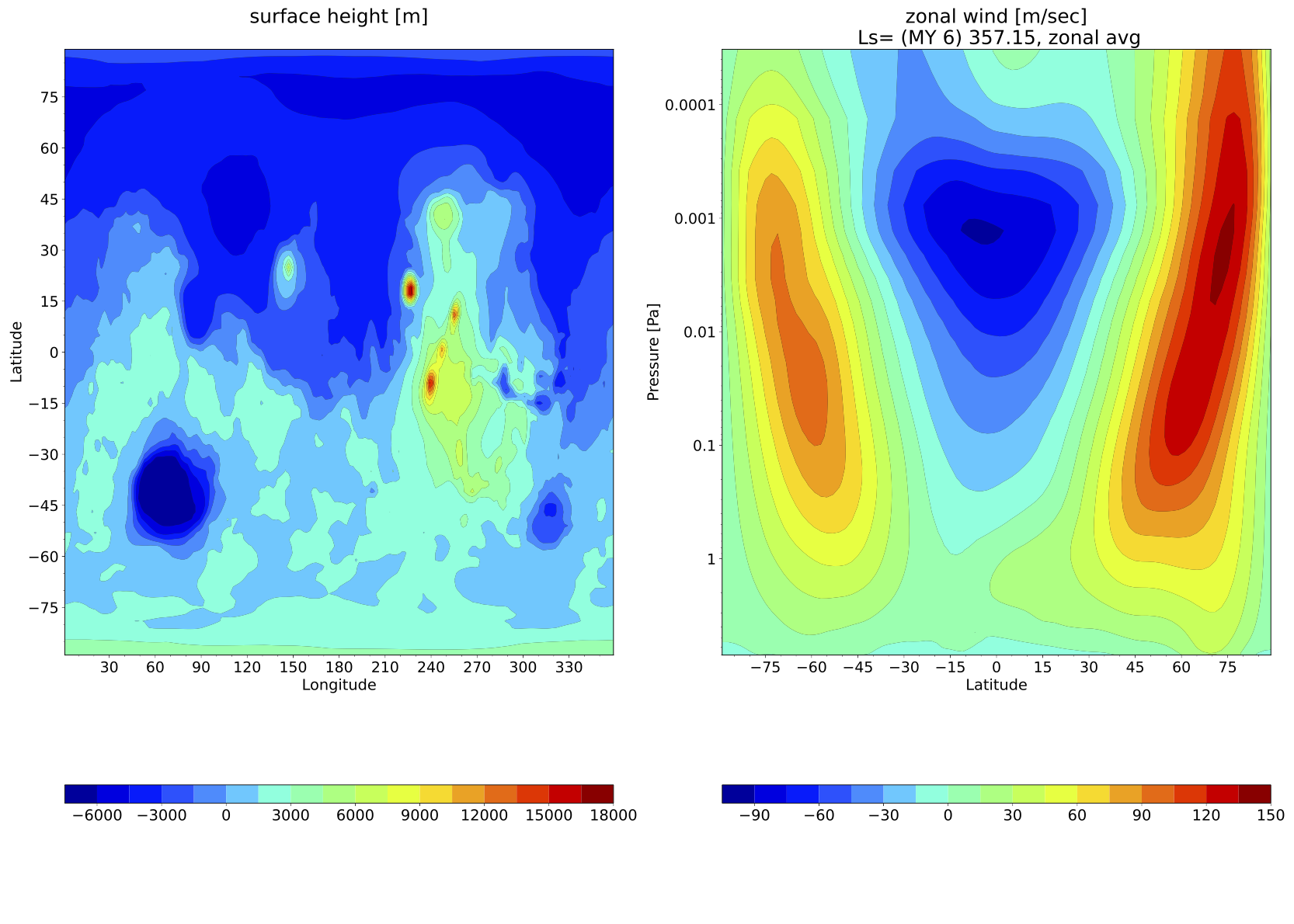
We’ll preserve the first two plots, but let’s define the sol number of the average and fixed files in the template itself so we don’t have to pass the [-d --date] argument every time:

# for the first plot (lon X lat topography):
Main Variable  = 03340.fixed.zsurf
# for the second plot (lat X lev zonal wind):
Main Variable  = 03340.atmos_average.ucomp

Now we can omit the date ([-d --date]) when we pass Custom.in to MarsPlot.

Custom Set 1 of 4: Zonal Mean Surface Plots Over Time

The first set of plots we’ll make are zonal mean surface fields over time: surface temperature, CO₂ ice, and wind stress.

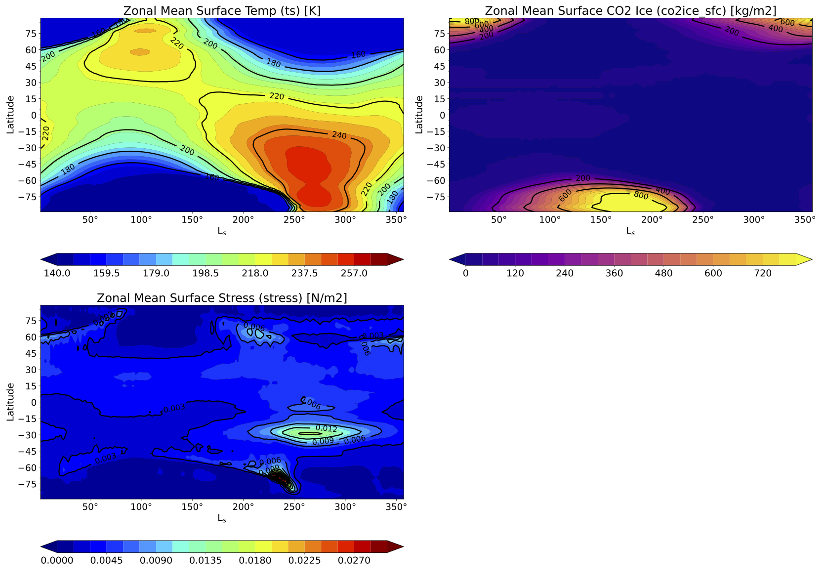
For each of the plots, source variables from the non-interpolated average file, 03340.atmos_average.nc.

For the surface temperature plot:

• Copy/paste the Plot 2D time X lat template above the Empty Templates line

• Set it to True

• Edit the title to Zonal Mean Sfc T [K]

• Set Main Variable = 03340.atmos_average.ts

• Edit the colorbar range: Cmin, Cmax = 140,270 → 140-270 Kelvin

• Set 2nd Variable = 03340.atmos_average.ts → for overplotted solid contours

• Explicitly define the solid contours: Contours Var 2 = 160,180,200,220,240,260

Let’s pause here and pass the Custom.in file to MarsPlot.

Type ESC-:wq to save and close the file. Then, pass it to MarsPlot:

(amescap)~$ MarsPlot Custom.in

Now, go to your local terminal tab and retrieve the PDF:

(local)~$ getpwd

Now we can open it and view our plot.

Go back to the cloud environment tab to finish generating the other plots on this page. Open Custom.in in vim:

(amescap)~$ vim Custom.in

HOLD ON`` and HOLD OFF arguments around the surface temperature plot. We will paste the other templates within these arguments to tell MarsPlot to put these plots on the same page.

Copy/paste the Plot 2D time X lat template plot twice more. Make sure to set the boolean to True.

For the surface CO2 ice plot:

• Set the title to Zonal Mean Sfc CO2 Ice [kg/m2]

• Set Main Variable = 03340.atmos_average.co2ice_sfc

• Edit the colorbar range: Cmin, Cmax = 0,800 → 0-800 kg/m2

• Set 2nd Variable = 03340.atmos_average.co2ice_sfc → solid contours

• Explicitly define the solid contours: Contours Var 2 = 200,400,600,800

• Change the colormap on the Axis Options line: cmap = plasma

For the surface wind stress plot:

• Set the title to Zonal Mean Sfc Stress [N/m2]

• Set Main Variable = 03340.atmos_average.stress

• Edit the colorbar range: Cmin, Cmax = 0,0.03 → 0-0.03 N/m2

Save and quit the editor (ESC-:wq) and pass Custom.in to MarsPlot:

(amescap)~$ MarsPlot Custom.in

Return to Part II: Plotting with CAP

---

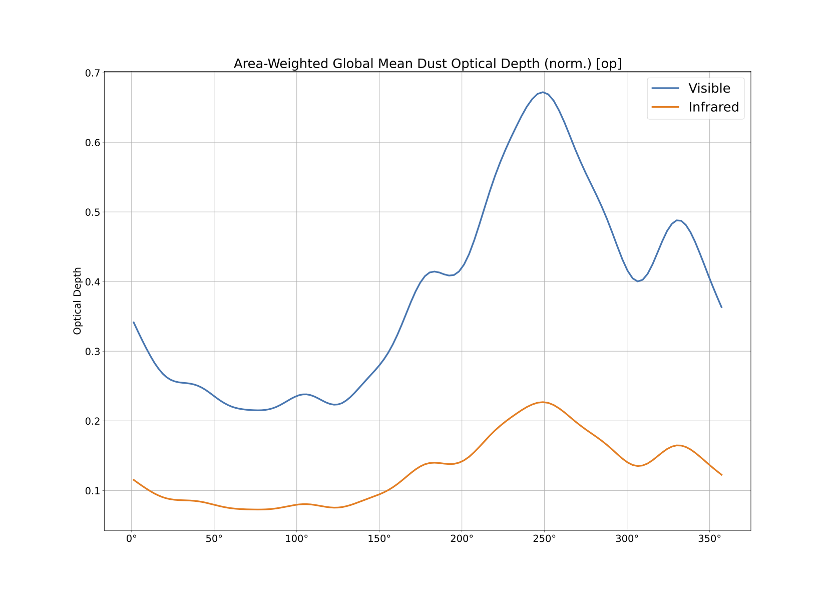
Custom Set 2 of 4: Global Mean Column-Integrated Dust Optical Depth Over Time

Now we’ll generate a 1D plot and practice plotting multiple lines on it.

Let’s start by setting up our 1D plot template:

• Write a new set of HOLD ON and HOLD OFF arguments.

• Copy/paste the Plot 1D template between them.

• Set the template to True.

Create the visible dust optical depth plot first:

• Set the title: Area-Weighted Global Mean Dust OD (norm.) [op]

• Edit the legend: Visible

The input to Main Variable is not so straightforward this time. We want to plot the normalized dust optical depth, which is dervied as follows:

normalized_dust_OD = opacity / surface_pressure * reference_pressure

The MGCM outputs column-integrated visible dust opacity to the variable taudust_VIS, surface pressure is saved as ps, and we’ll use a reference pressure of 610 Pa. Recall that element-wise operations are performed when square brackets [] are placed around the variable in Main Variable. Putting all that together, Main Variable is:

# ┌ norm. OD     ┌ opacity                         ┌ surface pressure       ┌ ref. P
Main Variable  = [03340.atmos_average.taudust_VIS]/[03340.atmos_average.ps]*610

To finish up this plot, tell MarsPlot what to do to the dimensions of taudust_VIS (time, lon, lat):

• Leave Ls 0-360 = AXIS to use ‘time’ as the X axis dimension.

• Set Latitude = all → average over all latitudes

• Set Lon +/-180  = all → average over all longitudes

• Set the Y axis label under Axis Options: axlabel = Optical Depth

The infrared dust optical depth plot is identical to the visible dust OD plot except for the variable being plotted, so duplicate the visible plot we just created. Make sure both templates are between HOLD ON and HOLD OFF Then, change two things:

• Change Main Variable from taudust_VIS to taudust_IR

• Set the legend to reflect the new variable (Legend = Infrared)

Save and quit the editor (ESC-:wq). pass Custom.in to MarsPlot:

(amescap)~$ MarsPlot Custom.in

Notice we have two separate 1D plots on the same page. This is because of the HOLD ON and HOLD OFF arguments. Without those, these two plots would be on separate pages. But how do we overplot the lines on top of one another?

Go back to the cloud environment, open Custom.in, and type ADD LINE between the two 1D templates.

Save and quit again, pass it through MarsPlot, and retrieve the PDF locally. Now we have the overplotted lines we were looking for.

Return to Part II: Plotting with CAP

---

Custom Set 3 of 4: 50 Pa Temperatures at 3 AM and 3 PM

The first two plots are 3 AM and 3 PM 50 Pa temperatures at L_s=270. Below is the 3 PM - 3 AM difference.

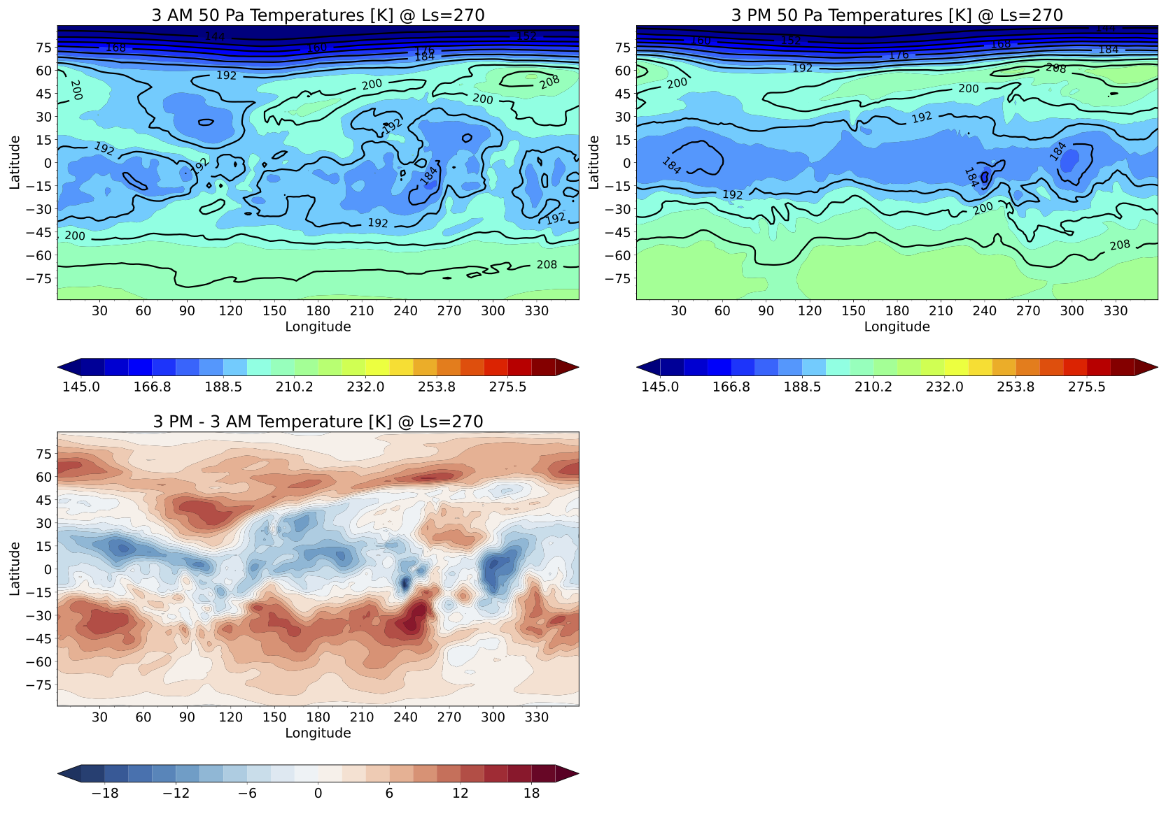
We’ll generate all three plots before passing Custom.in to MarsPlot, so copy/paste the Plot 2D lon X lat template *three times* between a set of HOLD ON and HOLD OFF arguments and set them to True.

For the first plot,

• Title it for 3 AM temperatures: 3 AM 50 Pa Temperatures [K] @ Ls=270

• Set Main Variable to temp and select 3 AM for the time of day using curly brackets:

Main Variable  = 03847.atmos_diurn_Ls265_275_T_pstd.temp{tod=3}

• Set the colorbar range: Cmin, Cmax = 145,290 → 145-290 K

• Set Ls 0-360 = 270 → southern summer solstice

• Set Level Pa/m = 50 → selects 50 Pa temperatures

• Set 2nd Variable to be identical to Main Variable

Now, edit the second template for 3 PM temperatures the same way. The only differences are the:

• Title: edit to reflect 3 PM temperatures

• Time of day selection: for 3 PM, {tod=15} *change this for ``2nd Variable`` too!*

For the difference plot, we will need to use square brackets in the input for Main Variable in order to subtract 3 AM temperatures from 3 PM temperatures. We’ll also use a diverging colorbar to show temperature differences better.

• Set the title to 3 PM - 3 AM Temperature [K] @ Ls=270

• Build Main Variable by subtracting the 3 AM Main Variable input from the 3 PM Main variable input:

Main Variable = [03847.atmos_diurn_Ls265_275_T_pstd.temp{tod=15}]-[03847.atmos_diurn_Ls265_275_T_pstd.temp{tod=3}]

• Center the colorbar at 0 by setting Cmin, Cmax = -20,20

• Like the first two plots, set Ls 0-360 = 270 → southern summer solstice

• Like the first two plots, set Level Pa/m = 50 → selects 50 Pa temperatures

• Select a diverging colormap in Axis Options: cmap = RdBu_r

Save and quit the editor (ESC-:wq). pass Custom.in to MarsPlot, and pull it to your local computer:

(amescap)~$ MarsPlot Custom.in

Return to Part II: Plotting with CAP

---

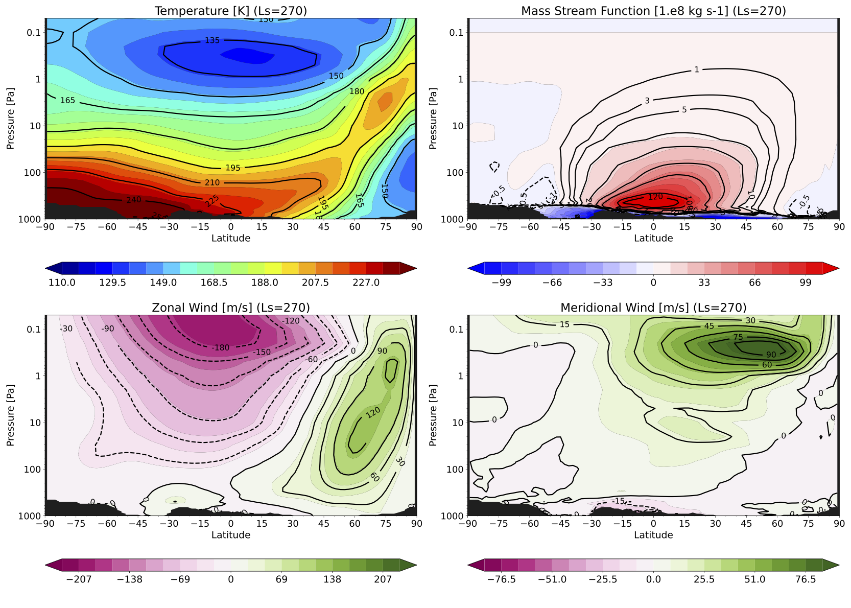
Custom Set 4 of 4: Zonal Mean Circulation Cross-Sections

For our final set of plots, we will generate four cross-section plots showing temperature, zonal (U) and meridional (V) winds, and mass streamfunction at L_s=270.

Begin with the usual 3-step process:

1. Write a set of HOLD ON and HOLD OFF arguments

2. Copy-paste the Plot 2D lat X lev template between them

3. Set the template to True

Since all four plots are going to have the same X and Y axis ranges and time selection, let’s edit this template before copying it three more times:

• Set Ls 0-360 = 270

• In Axis Options, set Lat = [-90,90]

• In Axis Options, set level[Pa/m] = [1000,0.05]

Now copy/paste this template three more times. Let the first plot be temperature, the second be mass streamfunction, the third be zonal wind, and the fourth be meridional wind.

For temperature:

Title          = Temperature [K] (Ls=270)
Main Variable  = 03847.atmos_average_Ls265_275_pstd.temp
Cmin, Cmax     = 110,240
...
2nd Variable   = 03847.atmos_average_Ls265_275_pstd.temp

For streamfunction, define explicit solid contours under Contours Var 2 and set a diverging colormap.

Title          = Mass Stream Function [1.e8 kg s-1] (Ls=270)
Main Variable  = 03847.atmos_average_Ls265_275_pstd.msf
Cmin, Cmax     = -110,110
...
2nd Variable   = 03847.atmos_average_Ls265_275_pstd.msf
Contours Var 2 = -5,-3,-1,-0.5,1,3,5,10,20,40,60,100,120
# set cmap = bwr in Axis Options

For zonal and meridional wind, use the dual-toned colormap PiYG.

Title          = Zonal Wind [m/s] (Ls=270)
Main Variable  = 03847.atmos_average_Ls265_275_pstd.ucomp
Cmin, Cmax     = -230,230
...
2nd Variable   = 03847.atmos_average_Ls265_275_pstd.ucomp
# set cmap = PiYG in Axis Options

Title          = Meridional Wind [m/s] (Ls=270)
Main Variable  = 03847.atmos_average_Ls265_275_pstd.vcomp
Cmin, Cmax     = -85,85
...
2nd Variable   = 03847.atmos_average_Ls265_275_pstd.vcomp
# set cmap = PiYG in Axis Options

Save and quit the editor (ESC-:wq). pass Custom.in to MarsPlot, and pull it to your local computer:

(amescap)~$ MarsPlot Custom.in

Return to Part II: Plotting with CAP

---

End Credits

This concludes the practical exercise portion of the CAP tutorial. Please feel free to use these exercises as a reference when using CAP the future!

Written by Courtney Batterson, Alex Kling, and Victoria Hartwick. This document was created for the NASA Ames MGCM and CAP Tutorial held virtually November 13-15, 2023.

Questions, comments, or general feedback? `Contact us <https://forms.gle/2VGnVRrvHDzoL6Y47>`_.

Return to Table of Contents